No8 - PINNs
Fecha: 06/05/2026
Optimización con restricciones y dualidad lagrangiana ¶ Muchos de los problemas que hasta ahora trabajamos parecieran tratar de minimizar la función de costo sin restricciones ; por ejemplo, cuadrados mínimos:
min θ L ( θ , y ) = min θ ∑ i = 1 N ∥ ∥ y i − x ( t i , θ ) ∥ ∥ 2 2 ( 1 ) \min_{\theta} \mathcal{L} (\theta,y)=\min_{\theta}\sum_{i=1}^{N} \left\|\left\| y_i - x(t_i,\theta) \right\| \right\|_2^2 \qquad (1) θ min L ( θ , y ) = θ min i = 1 ∑ N ∥ ∥ y i − x ( t i , θ ) ∥ ∥ 2 2 ( 1 ) donde L \mathcal{L} L
Podemos reescribir esto como un problema con restricciones , dejando a x x x
min θ , x ∑ i = 1 N ∥ ∥ y i − x ( t i ) ∥ ∥ 2 2 sujeto a { d x d t = f ( x , t , θ ) x ( t 0 ) = x 0 \min_{\theta,x}
\sum_{i=1}^{N}
\left\|\left\| y_i - x(t_i) \right\| \right\|_2^2
\quad
\text{sujeto a}
\quad
\begin{cases}
\dfrac{dx}{dt} = f(x,t,\theta) \\
x(t_0)=x_0
\end{cases} θ , x min i = 1 ∑ N ∥ ∥ y i − x ( t i ) ∥ ∥ 2 2 sujeto a ⎩ ⎨ ⎧ d t d x = f ( x , t , θ ) x ( t 0 ) = x 0 Es decir, estamos convirtiendo
min θ f ( x ( θ ) ) \min_{\theta} f(x(\theta)) θ min f ( x ( θ )) en
min θ , x f ( x , θ ) sujeto a G ( x , θ ) = 0 \min_{\theta,x} f(x,\theta)
\quad
\text{sujeto a}
\quad
G(x,\theta)=0 θ , x min f ( x , θ ) sujeto a G ( x , θ ) = 0 Si uno puede invertir G ( x , θ ) G(x,\theta) G ( x , θ ) x = x ( θ ) x=x(\theta) x = x ( θ )
En este caso,
G ( x , θ ) = [ d u d t − f ( u , t , θ ) u ( t 0 ) − u 0 ] = 0 G(x,\theta)=
\begin{bmatrix}
\dfrac{du}{dt} - f(u,t,\theta) \\
u(t_0)-u_0
\end{bmatrix}
=0 G ( x , θ ) = [ d t d u − f ( u , t , θ ) u ( t 0 ) − u 0 ] = 0 Esto se hace con el solver numérico.
La forma más general del problema de optimización puede escribirse como:
min θ f ( θ ) \min_{\theta} f(\theta) θ min f ( θ ) sujeto a
{ g ( θ ) = 0 h ( θ ) ≤ 0 \begin{cases}
g(\theta)=0 \\
h(\theta)\leq 0
\end{cases} { g ( θ ) = 0 h ( θ ) ≤ 0 La diferencia entre resolver estos problemas con y sin restricciones es debido a la dualidad lagrangiana.
Dualidad lagrangiana ¶ La dualidad lagrangiana toma un problema con restricciones y lo transforma en uno sin restricciones mediante mediante el metodo de los multiplicadores de Lagrange.
Se define el lagrangiano:
L ( θ , λ , ν ) = f ( θ ) + λ g ( θ ) + ν h ( θ ) \mathcal{L}(\theta,\lambda,\nu)
= f(\theta)
+
\lambda g(\theta)
+
\nu h(\theta) L ( θ , λ , ν ) = f ( θ ) + λ g ( θ ) + ν h ( θ ) donde:
Imaginemos un problema sin restricciones h h h Boyd & Vandenberghe (2004)
max λ min θ L ( θ , λ ) = min θ max λ L ( θ , λ ) \max_{\lambda}\min_{\theta}\mathcal{L}(\theta,\lambda)=\min_{\theta}\max_{\lambda}\mathcal{L}(\theta,\lambda) λ max θ min L ( θ , λ ) = θ min λ max L ( θ , λ ) Ejemplo: Lasso ¶ Consideremos el problema de optimización:
min θ ∥ ∥ y − x θ ∥ ∥ 2 2 + λ ∥ ∥ θ ∥ ∥ 1 \min_{\theta}
\left\| \left\| y - x \theta \right\| \right\|_2^2
+
\lambda \left\| \left\| \theta \right\| \right\|_1 θ min ∥ ∥ y − x θ ∥ ∥ 2 2 + λ ∥ ∥ θ ∥ ∥ 1 donde:
el primer término corresponde al error de ajuste,
el segundo término penaliza la complejidad del modelo (en este caso, prefiere soluciones esparsas).
Recordemos que
∥ ∥ θ ∥ ∥ 1 = ∑ i = 1 p ∥ ∥ θ i ∥ ∥ \left\| \left\| \theta \right\| \right\|_1=\sum_{i=1}^{p} \left\| \left\| \theta_i \right\| \right\| ∥ ∥ θ ∥ ∥ 1 = i = 1 ∑ p ∥ ∥ θ i ∥ ∥ Entonces puede mostrarse que el θ ∗ \theta^\ast θ ∗
θ ∗ = arg min θ ∥ ∥ y − x θ ∥ ∥ 2 2 + λ ∥ ∥ θ ∥ ∥ 1 \theta^\ast=
\arg\min_{\theta}
\left\| \left\| y- x\theta \right\| \right\|_2^2
+
\lambda \left\| \left\| \theta \right\| \right\|_1 θ ∗ = arg θ min ∥ ∥ y − x θ ∥ ∥ 2 2 + λ ∥ ∥ θ ∥ ∥ 1 puede reinterpretarse como
θ ∗ = arg min θ ∥ ∥ y − x θ ∥ ∥ 2 2 sujeto a ∥ ∥ θ ∥ ∥ 1 ≤ C ( λ ) \theta^\ast = \arg\min_{\theta} \left\| \left\| y-x\theta \right\| \right\|_2^2 \quad \text{sujeto a} \quad \left\| \left\| \theta \right\| \right\|_1 \leq C(\lambda) θ ∗ = arg θ min ∥ ∥ y − x θ ∥ ∥ 2 2 sujeto a ∥ ∥ θ ∥ ∥ 1 ≤ C ( λ ) Por lo cual, la dualidad lagrangiana nos asegura que un problema de minimización de un lagrangiano puede reescribirse como un problema de optimización con restricciones.
Notar que si nuestro λ → 0 \lambda \rightarrow 0 λ → 0 C → ∞ C \rightarrow \infty C → ∞ θ \theta θ C C C λ \lambda λ C C C
Problema relajado ¶ Hay posibilidad de “relajar” la función de costo con un factor ε \varepsilon ε
min θ , x L ( θ , x ) = ( 3 ) \min_{\theta,x} \mathcal{L}(\theta,x)= \qquad (3) θ , x min L ( θ , x ) = ( 3 ) sujeto a
∥ ∥ d x d t − f ( x , t , θ ) ∥ ∥ 2 ≤ ε ∀ t \left\| \left\| \frac{dx}{dt} - f(x,t,\theta) \right\| \right\|_2 \leq \varepsilon \qquad \forall t ∥ ∥ ∥ ∥ d t d x − f ( x , t , θ ) ∥ ∥ ∥ ∥ 2 ≤ ε ∀ t y
∥ ∥ x ( t 0 ) − u 0 ∥ ∥ 2 ≤ ε \left\| \left\| x(t_0)-u_0 \right\| \right\|_2 \leq \varepsilon ∥ ∥ x ( t 0 ) − u 0 ∥ ∥ 2 ≤ ε donde recuperamos el problema (1) si ε = 0 \varepsilon=0 ε = 0
min θ , x L ( θ , x ) + λ ε ∫ t 0 t 1 ∥ ∥ d x d t − f ( x , t , θ ) ∥ ∥ 2 2 d t ( 4 ) \min_{\theta,x} \mathcal{L}(\theta,x)+
\lambda_{\varepsilon}
\int_{t_0}^{t_1}
\left\| \left\|
\frac{dx}{dt}
-f(x,t,\theta) \right\| \right\|_2^2 dt \qquad (4) θ , x min L ( θ , x ) + λ ε ∫ t 0 t 1 ∥ ∥ ∥ ∥ d t d x − f ( x , t , θ ) ∥ ∥ ∥ ∥ 2 2 d t ( 4 ) El segundo término actúa como un término de regularización con derivadas (en el caso clásico de estadística esto corresponde a un “profiling”). Asimismo, vemos que si ε → 0 \varepsilon \rightarrow 0 ε → 0 λ ε → ∞ \lambda_\varepsilon \rightarrow \infty λ ε → ∞ “splines” o “smooth splines” , solo que allí se utilizan las derivadas segundas.
La ecuación (4) constituye el punto de partida para una PINN (Physics-Informed Neural Network ).
Las PINNs fueron introducidas recientemente por Raissi, Perdikaris y Karniadakis en el siguiente trabajo: Raissi et al. (2019)
Caso ODE ¶ La idea es agarrar el “profiling” y nuestras incógnitas a optimizar (x ( t ) x(t) x ( t ) x ( t ) x(t) x ( t )
donde β \beta β
β = [ W 1 , … , W n , b 1 , … , b n ] \beta = [W_1,\dots,W_n,b_1,\dots,b_n] β = [ W 1 , … , W n , b 1 , … , b n ] por lo cual, con esto, lo ponemos en la ecuación diferencial y optimizamos sobre los parámetros de la red neuronal. Por ejemplo, una red neuronal puede escribirse como:
x ( t ) = σ ( W 3 σ ( W 2 σ ( W 1 t ) + b 2 ) + b 3 ) x(t) = \sigma \left( W_3 \sigma \left( W_2 \sigma(W_1 t)+b_2\right) +b_3 \right) x ( t ) = σ ( W 3 σ ( W 2 σ ( W 1 t ) + b 2 ) + b 3 ) Para construir la función de costo necesitamos:
Poder evaluar x β ( t ) x_\beta(t) x β ( t ) t t t
Poder evaluar
d x β d t ∣ t = s \frac{dx_\beta}{dt}\Big|_{t=s} d t d x β ∣ ∣ t = s para cualquier s s s
Modo 1: PINN forward/directo ¶ En este caso, θ \theta θ
Una vez obtenida x ( t ) x(t) x ( t )
Tomamos puntos de prueba:
t 0 < z 1 < z 2 < ⋯ < z k < ⋯ < t 1 t_0 < z_1 < z_2 < \dots < z_k < \dots < t_1 t 0 < z 1 < z 2 < ⋯ < z k < ⋯ < t 1 y definimos la función de costo:
min β ∥ ∥ x ( t 0 ) − x 0 ∥ ∥ 2 2 + λ ~ ∑ k = 1 K ∥ ∥ ( d x β d t − f ( x , t , θ ) ) t = x k ∥ ∥ 2 \min_{\beta} \left\| \left\| x(t_0)-x_0\right\| \right\|_2^2 + \tilde{\lambda} \sum_{k=1}^{K} \left\| \left\| \left( \frac{dx_\beta}{dt} - f(x,t,\theta) \right)_{t=x_k} \right\| \right\|^2 β min ∥ ∥ x ( t 0 ) − x 0 ∥ ∥ 2 2 + λ ~ k = 1 ∑ K ∥ ∥ ∥ ∥ ( d t d x β − f ( x , t , θ ) ) t = x k ∥ ∥ ∥ ∥ 2 La suma actúa como una aproximación de la integral.
Esto es equivalente a utilizar una red neuronal como solver numérico.
Ejemplo: ecuación del calor ¶ Consideremos:
x ∈ R n , t ∈ R , ( n = 1 , 2 , 3 ) x \in \mathbb{R}^n,
\qquad
t \in \mathbb{R},
\qquad
(n=1,2,3) x ∈ R n , t ∈ R , ( n = 1 , 2 , 3 ) La ecuación del calor es:
∂ u ∂ t − D ∇ 2 u = 0 \frac{\partial u}{\partial t} - D \nabla^2 u = 0 ∂ t ∂ u − D ∇ 2 u = 0 donde D D D ∇ 2 = ∂ ∂ x + ∂ ∂ y + ∂ ∂ z \nabla^2 = \frac{\partial}{\partial x} + \frac{\partial}{\partial y} + \frac{\partial}{\partial z} ∇ 2 = ∂ x ∂ + ∂ y ∂ + ∂ z ∂
La ecuación debe satisfacerse para:
∀ x ∈ Ω , ∀ t ∈ [ t 0 , t 1 ] \forall x\in\Omega,
\qquad
\forall t\in[t_0,t_1] ∀ x ∈ Ω , ∀ t ∈ [ t 0 , t 1 ] con la condición de borde:
u ( x , t ) = u B ( x , t ) ∀ x ∈ ∂ Ω u(x,t)=u_B(x,t)
\qquad
\forall x\in\partial\Omega u ( x , t ) = u B ( x , t ) ∀ x ∈ ∂ Ω y su condición inicial:
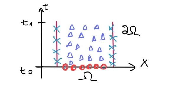
u ( x , t 0 ) = u 0 ( x ) u(x,t_0)=u_0(x) u ( x , t 0 ) = u 0 ( x ) Vamos a considerar una parametrización para el borde espacial, otra para la condición inicial y finalmente para los puntos del interior. Podemos visualizar esto en el siguiente diagrama
Las cruces simbolizan la parametrización del borde espacial, los círculos el borde temporal, y los triángulos los puntos del interior.
Función de costo total ¶ La función de costo a minimizar sobre los parámetros β \beta β
min β λ 1 ∑ i = 1 K 1 ∥ ∥ u β ( t 0 , x i I ) − u 0 ( x i I ) ∥ ∥ 2 + λ 2 ∑ j = 1 K 2 ∥ ∥ u β ( t j B , x j B ) − u B ( t j B , x j B ) ∥ ∥ 2 + λ 3 ∑ m = 1 K 3 ∥ ∥ G [ u β ] ∣ t M , x M ∥ ∥ 2 2 \min_{\beta} \; \lambda_1 \sum_{i=1}^{K_1} \left\| \left\| u_\beta(t_0, x_i^I) - u_0(x_i^I) \right\| \right\|^2 + \lambda_2 \sum_{j=1}^{K_2} \left\| \left\| u_\beta(t_j^B, x_j^B) - u_B(t_j^B, x_j^B) \right\| \right\|^2 + \lambda_3 \sum_{m=1}^{K_3} \left\| \left\| \mathcal{G}[u_\beta] \Big|_{t_M, x_M} \right\| \right\|_2^2 β min λ 1 i = 1 ∑ K 1 ∥ ∥ ∥ ∥ u β ( t 0 , x i I ) − u 0 ( x i I ) ∥ ∥ ∥ ∥ 2 + λ 2 j = 1 ∑ K 2 ∥ ∥ ∥ ∥ u β ( t j B , x j B ) − u B ( t j B , x j B ) ∥ ∥ ∥ ∥ 2 + λ 3 m = 1 ∑ K 3 ∥ ∥ ∥ ∥ G [ u β ] ∣ ∣ t M , x M ∥ ∥ ∥ ∥ 2 2 ≡ L inicial + L borde + L f ı ˊ sico \equiv \mathcal{L}_{\text{inicial}} + \mathcal{L}_{\text{borde}} + \mathcal{L}_{\text{físico}} ≡ L inicial + L borde + L f ı ˊ sico Los círculos representan u 0 ( x i I ) u_0(x_i^I) u 0 ( x i I ) I I I
Las cruces a u B ( t j B , x j B ) u_B(t_j^B, x_j^B) u B ( t j B , x j B ) B B B
Los triángulos representan a G [ u β ] ∣ t M , x M \mathcal{G}[u_\beta] \Big|_{t_M, x_M} G [ u β ] ∣ ∣ t M , x M M M M
Arquitectura de la red y funciones de costo ¶ La red neuronal recibe como entradas t , x 1 , … , x n t, x_1, \ldots, x_n t , x 1 , … , x n u β ( t , x ) u_\beta (t,x) u β ( t , x )
Operación Resultado Función de costo asociada Id \text{Id} Id u β u_\beta u β L inicial \mathcal{L}_{\text{inicial}} L inicial ∂ ∂ t \frac{\partial}{\partial t} ∂ t ∂ ∂ u β ∂ t \dfrac{\partial u_\beta}{\partial t} ∂ t ∂ u β L borde \mathcal{L}_{\text{borde}} L borde ∇ \nabla ∇ ∇ u β \nabla u_\beta ∇ u β L f ı ˊ sico \mathcal{L}_{\text{físico}} L f ı ˊ sico
Las tres funciones de costo se combinan en:
L TOTAL = L inicial + L borde + L f ı ˊ sico \mathcal{L}_{\text{TOTAL}} = \mathcal{L}_{\text{inicial}} + \mathcal{L}_{\text{borde}} + \mathcal{L}_{\text{físico}} L TOTAL = L inicial + L borde + L f ı ˊ sico Objetivo del modo Forward ¶ ⟹ min β L TOT ( β ) ≃ 0 y u β soluci o ˊ n a la ecuaci o ˊ n \implies \min_{\beta} \, \mathcal{L}_{\text{TOT}}(\beta) \simeq 0 \quad \text{y} \quad u_\beta \text{solución a la ecuación} ⟹ β min L TOT ( β ) ≃ 0 y u β soluci o ˊ n a la ecuaci o ˊ n Hasta aquí todo es modo Forward.
PINNs Modo 2: Inverso ¶ ¡Este es el uso verdadero de una PINN! El modo “forward” es mas de juguete que otra cosa.
Problema ¶ Dados los datos observados [ u obs ( t i , x i ) ] i = 1 N \left[u^{\text{obs}}(t_i, x_i)\right]_{i=1}^{N} [ u obs ( t i , x i ) ] i = 1 N recuperar D = D ( x ) D = D(x) D = D ( x ) x x x
Idea ¶ Se desarrolla D D D Red Neuronal con parámetros β 2 \beta_2 β 2
L emp = λ ∑ i = 1 N ∥ ∥ u β 1 ( x i , t i ) − u obs ( t i , x i ) ∥ ∥ 2 2 \mathcal{L}_{\text{emp}} = \lambda \sum_{i=1}^{N} \left\| \left\| u_{\beta_1}(x_i, t_i) - u^{\text{obs}}(t_i, x_i) \right\| \right\|_2^2 L emp = λ i = 1 ∑ N ∥ ∥ ∥ ∥ u β 1 ( x i , t i ) − u obs ( t i , x i ) ∥ ∥ ∥ ∥ 2 2 Ahora la arquitectura involucra dos redes ¶ Se tienen dos redes con parámetros distintos:
Red β 1 \beta_1 β 1 : aproxima la solución u β 1 ( t , x ) u_{\beta_1}(t, x) u β 1 ( t , x )
Red β 2 \beta_2 β 2 : aproxima la difusividad D β 2 ( x ) → R D_{\beta_2}(x) \to \mathbb{R} D β 2 ( x ) → R x x x
Operación sobre u β 1 u_{\beta_1} u β 1 Resultado Función de costo asociada Id \text{Id} Id u β 1 u_{\beta_1} u β 1 L inicial, borde, emp ı ˊ rica \mathcal{L}_{\text{inicial, borde, empírica}} L inicial, borde, emp ı ˊ rica ∂ ∂ t \frac{\partial}{\partial t} ∂ t ∂ ∂ u β 1 ∂ t \dfrac{\partial u_{\beta_1}}{\partial t} ∂ t ∂ u β 1 L f ı ˊ sica \mathcal{L}_{\text{física}} L f ı ˊ sica ∇ \nabla ∇ ∇ u β 1 \nabla u_{\beta_1} ∇ u β 1 L f ı ˊ sica \mathcal{L}_{\text{física}} L f ı ˊ sica
Operación sobre D β 1 D_{\beta_1} D β 1 Resultado Función de costo asociada Id \text{Id} Id D β 1 D_{\beta_1} D β 1 L f ı ˊ sica \mathcal{L}_{\text{física}} L f ı ˊ sica
La función de costo empírica también se incorpora a L TOTAL \mathcal{L}_{\text{TOTAL}} L TOTAL
Parámetros a optimizar ¶ β = [ β 1 , β 2 ] \beta = [\beta_1, \beta_2] β = [ β 1 , β 2 ] Se minimiza la función de costo total conjuntamente sobre β 1 \beta_1 β 1 β 2 \beta_2 β 2 u β 1 u_{\beta_1} u β 1 y D β 2 D_{\beta_2} D β 2
Boyd, S., & Vandenberghe, L. (2004). Convex optimization . Cambridge university press. Raissi, M., Perdikaris, P., & Karniadakis, G. E. (2019). Physics-informed neural networks: A deep learning framework for solving forward and inverse problems involving nonlinear partial differential equations. Journal of Computational Physics , 378 , 686–707. 10.1016/j.jcp.2018.10.045